
Become the master of sorter and belt with math.
Guide to Math Analysis of Sorter Efficiency on Belt
Introduction
Sorter Efficiency is affected by the item/slot availability of the source and destination spot. This is mostly complicated when sorter is place on a belt/belts.
For example, when the target grid of a sort is a belt that is most full, then we will observe that the sorter has a hard time finding an empty slot to deliver the item, resulting in a much lower efficiency. The same effect would be observed when sorting is trying to pick up an item from a mostly empty belt.
We provide a formal math analysis of sorter efficiency on belt and some handy formulas for in game calculation/estimation.
Background
First let’s review the current game basics:
Type: Sorter – Belt
- MK1: 1.5/s – 4/s
- MK2: 3/s – 12/s
- MK3: 6/s – 30/s
Note: The sorter speed in the table is for 1-grid-span. The actual speed is divide by the grid span (2 or 3). For example. MK2 sorter at 2-grid-span is 1.5/s, the same as MK1. And it becomes 1/s at 3-grid-span, less than MK1.
For the rest of the doc, we will always use the 1-grid-span value for example calculations.
A little bit less obviously, a belt actually has 2 slots per tile. If we build a belt of 100 tiles, we will observe that the belt can hold about 200 items in it (it’s not exactly 200 because the end tiles and the turn tiles are slightly different than the straight line middle tiles). Belt speed is actually measured in belt slots instead of tiles. In other words, in 1 second a item on MK1 belt travels 6 slots, which is 3 tiles, not 6 tiles. This is easy to verify. If you make a close loop belt of 60 tiles, put a single item on it, and measure the time it completes one loop. It will be 20 seconds instead of 10.
From now on we will use b/s (as belt slots/second) for the unit of belt speed, to not confuse it with tiles/second, which perhaps mostly people mistakenly assume. Also we will use the “number of slots” length to measure the length of a belt, not the tile length.
Belt Slots and Sorter Delay
To make it easier for the math to kick in, we first define alternative quantities to measure things.
Model a running belt
This is straightforward. If we watch the belt running, it has belt slots passing through any given point one after another, at its speed. If we index the belt slots with natural numbers, we will see that the following two events happened exactly 1 second apart:
- A. Slot 0 is right under a sorter
- B. Slot N is right under the same sorter
Where N equals to the belt speed.
We will then see that after another second, Slot 2N is right under the same sorter.
Sorter Delay
To investigate the interaction between sorter and belt, it is easier if we use sorter delay instead of speed.
Sorter Delay = Belt Speed/Sorter Speed
For example, MK1 sorter with MK1 belt gives us:
Sorter Delay = (6b/s) / (1.5/s) = 4b
This means the sorter delay for MK1 sorter on MK1 belt is 4 belt slots. You probably have already observed that if we use a single MK1 sorter to deliver items to an empty MK1 belt, the items will be placed on every 4th slots, like slot 0, 4, 8, 12…
Extended Sorter Delay and Efficiency
When a sorter is trying to deliver items to a belt that is already filled with some items, things get complicated. Imagine the sorter carries the item and reach out on top of the belt but unable to deliver, because the slot below it is filled. What does it do? It simply waits and the belt passes by. At the next slot, if it’s empty, the delivery succeeds. Otherwise it waits again. Eventually it will find an empty lot and make it happen, as long as the belt is not completely full. However, it will take some waiting time.
We define
Wait Time : The number of belt slots it takes for a ready-at-destination sorter to wait until it can actually deliver
Note that this is called “time” but it’s not measured in seconds but in belt slots. If you are interested in the actual time, you can always divide it by belt speed. But as you can see below, it is more convenient to use this unit.
We then define
Extended Sorter Delay = Sorter Delay + Wait Time
As you might guess, the actual sorter speed can be calculated in the following way:
Actual Sorter Speed = Belt Speed / Extended Sorter Delay
Or if we would like to compare it with the original value:
Actual Sorter Speed = Sorter Speed * (Sorter Delay / Extended Sorter Delay)
Then we can define the efficiency as:
Efficiency = Actual Sorter Speed / Sorter Speed = Sorter Delay / Extended Sorter Delay
For example, a Sorter with a delay of 4 and waiting time of 2 will be running at 4/(4+2) = 66.7% efficiency.
Probability vs Expected Delay
Something we didn’t talk about in the last section: The Wait Time, and as a result the Extended Sorter Delay, are not fixed numbers. They can be considered random variables which can take different values at different trials.
In Sync Belt
Imagine an empty MK1 belt running through 4 MK1 sorters (they don’t need to be adjacent). Once the sorters start to work, the first sorter can always deliver without waiting, so it’s Wait Time is always 0 and Extended Sorter Delay is always 4. It will then deliver items to Slot 0, 4, 8, 12… The second sorter, while it might need to wait one slot, it will then deliver at 1, 5, 7, 11… The same holds for the third and the fourth sorter. They might experience waiting at the first delivery attempt, all subsequent delivery are then “in sync” and requires no waiting.
In this situation, the sorters will have max efficiency except maybe the first delivery, if the belt is not full.
Random Belt
Now imagine another empty MK1 belt, getting filled and partially emptied by various different mechanisms (different types of sorters, splitters, belt merge). Some of them might depend on other factors, like if another belt happens to have produce, or a assembler finishes work, or a storage is empty or not. In this case, it is increasing (as the belt length and systems it touches) unlikely that the items placed on the belt is in sync. We can then assume the belt slots are completely random variables.
One way to model it:
Random Belt Slots Model:
Each belt slot has a probability of p to be empty, independently.
Or in other words, the belt is (1-p)*100% filled, or p*100% empty.
For example a long belt with 2000 slots and with 800 items on it, the belt is 40% filled and 60% empty, the chance that each slot has an item will be 0.4.
Some elementary school math will tell us that with such a random model, the expected waiting time would be:
E(Wait Time) = 1/p – 1
For an completely empty belt p is 1 and the Wait Time naturally goes to 0.
For an almost full belt p is close to 0 and so Wait Time goes very large.
We can express the estimated efficiency, using expected Wait Time:
Estimated efficiency = Sorter Delay / E(Extended Sorter Delay) = Sorter Delay / (Sorter Delay + E(Wait Time)) = 1 / (1 + a)
In which the a factor is
a = (1/p – 1) / Sorter Delay
A-Factor Estimation
A-factor provides an easy way for us to estimate values. Given the emptiness of the belt, we can calculate the a factor thus the efficiency quickly, or vice versa.
For example, to get half efficiency we need a A-factor of 1. For Sorter Delay of 4, this means p = 1/5. That is, a MK1 sorter delivering to a MK1 belt with 20% emptiness, will run at 50% efficiency. You might then wonder, what if I change the MK1 sorter into a MK2 sorter? Let’s do the math:
- p = 1/5
- Sorter Delay = 2
- a = 2
- Estimated Efficiency = 1/3
It’s lower! Note the Actual Sorter speed is still faster, as it changes from 1.5 * 1/2 = 0.75 to 3 * 1/3 = 1. However it no longer a two times improvement.
Alternatively, with the same emptiness of 1/5, if we switch the belt from MK1 to MK2 but keep the MK1 sorter, that gives us:
- p = 1/5
- Sorter Delay = 8
- a = 1/2
- Estimated Efficiency = 2/3
This gives us a Actual Sorter Speed of 1.5 * 2/3 = 1, the same as changing the sorter.
Expand the Scope of the Fomula
Our original formulas are for delivering an item to a partially filled belt. However, it would naturally apply to the case of picking up items from the belt as well. Simply change the definition of p into fullness instead of emptiness, everything else is the same.
Taking a similar example, to get half efficiency we need a A-factor of 1. For Sorter Delay of 4, this means p = 1/5. That is, a MK1 sorter picking up items from a MK1 belt with 20% fullness, or, 80% emptiness, will run at 50% efficiency.
Even more fancy, our formula can be used on mixed items, when sorters has filter set. Imagine a belt filled with 40% iron, 30% magnet and 20% copper with 10% empty, a sorter filtered to pick iron will run at efficiency calculated with a p = 40%, as that’s what the sorter cares. If instead the sorter is filtered to pick magnet, then p = 30%. Copper for p = 20% and delivery item for p = 10%.
Fancy Application: The Automatic Load Balance on Belt
Some of you might have already stopped reading this guide, or at least wondered what is all the point to figure this math out. Well, here comes a fancy application:
Suppose we build a long, large loop belt to have mixed items running around (The main bus is an example of a large loop, but so far I haven’t see anyone make it to work with mixed items), can we control the percentage of each item on the belt, automatically. The answer is yes!
Starting with a simple setup:
The belt loop only has one place to “upload” iron into it and one place to “download” iron from it, let’s define some variables:
- Upload Sorter Delay = u
- Download Sorter Delay = d
- Belt Emptiness = m
- The ratio of iron filled in the loop = r
Now what happens when to the percentage of iron in the loop?
Well, we can have this “balance condition” equation:
- Estimated Actual Upload Speed = Estimated Actual Download Speed
- =>
- E(Extended Upload Sorter Delay) = E(Extended Download Sorter Delay)
Put the variables we defined above in:
- u + 1/m – 1 = d + 1/r – 1
- =>
- 1/r = 1/m + (u – d)
Once built, u – d becomes a constant which can be called Delay Diff.
When upload and download sorter has the same nominal speed, Delay Diff is 0, then then balance condition becomes that iron ratio on the belt is the same as empty ratio. If the belt only has iron then they are both 1/2. If the belt has N types of items all with 0 Delay Diff, then they each take 1/(1+N) in the belt and the last 1/(1+N) is empty.
A fast upload (thus smaller u) and slower download means a negative Delay Diff, which means 1/r will be smaller than 1/m, therefore r bigger than m. And vice versa.
For example, a MK1 belt with MK1 sorter for uploading and MK2 sorter for downloading, we will have Sorter Diff = 2. If there are only iron in the belt we can solve equations to find that we will end up with rough 71% emptiness and 29% iron on the belt.
The truly amazing part is that this will automatically balance itself. When there are too many irons on the belt (thus a bigger r), the download becomes faster and it will reduce the iron number. When there are too many empty spots on the belt, then the upload speed goes faster and it will reduce the emptiness.
Simple Examples
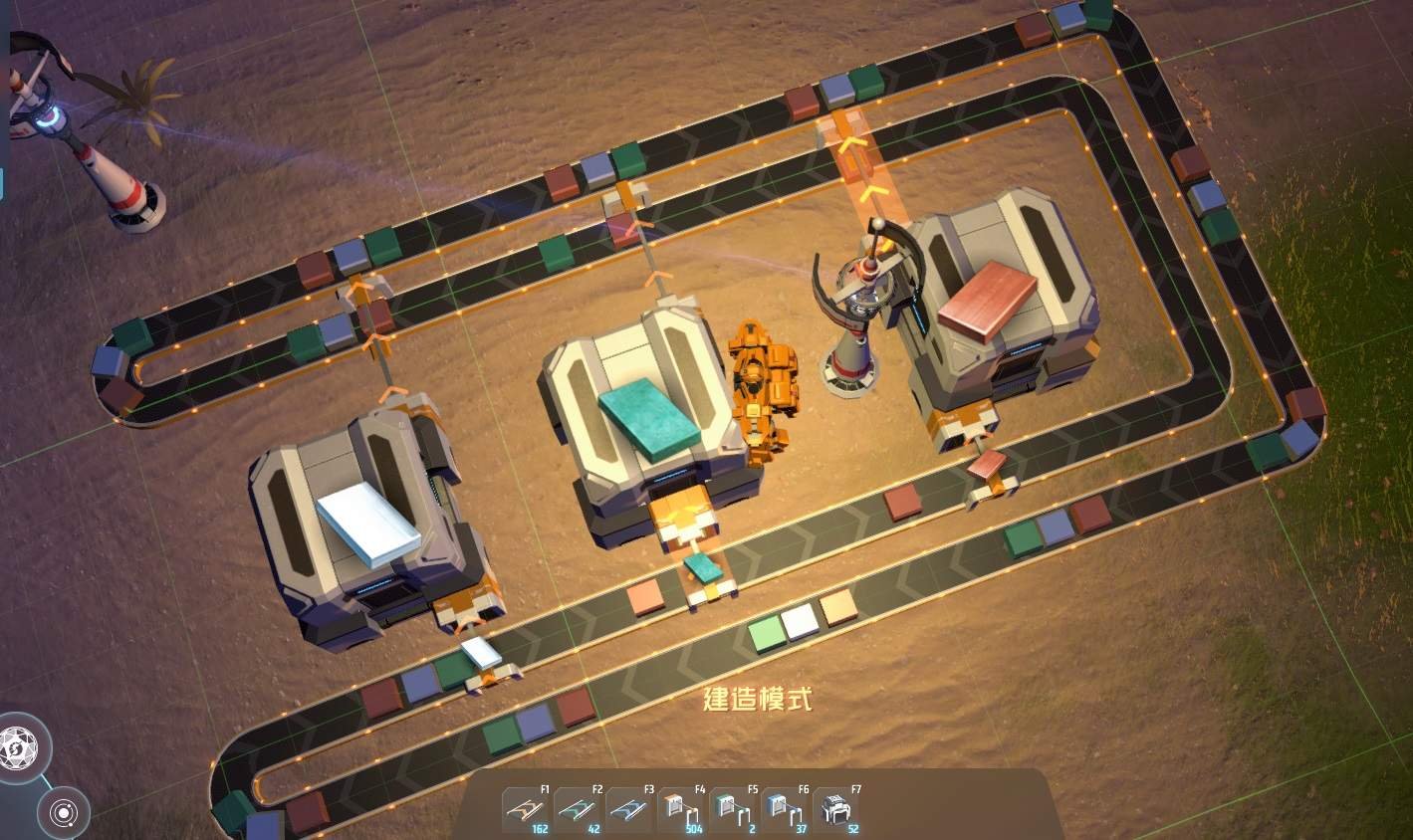
Here I built a simple small loop with 3 types of items mixed up.
By choosing different types of Upload/Download Sorter I can control the percentage of each items in the loop to reach some balance.
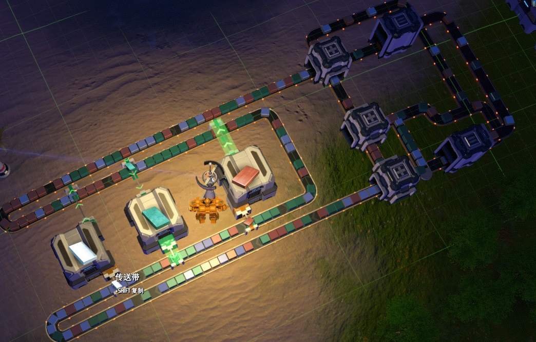
Download Heavy:
Upload Heavy:

You might notice that the items are no longer random and they form some kind of pattern quickly.
Mixed with randomizer:
Production Auto Stopper
Production can be auto stopped using a T joint trick, combined with the upload/download speed balance:
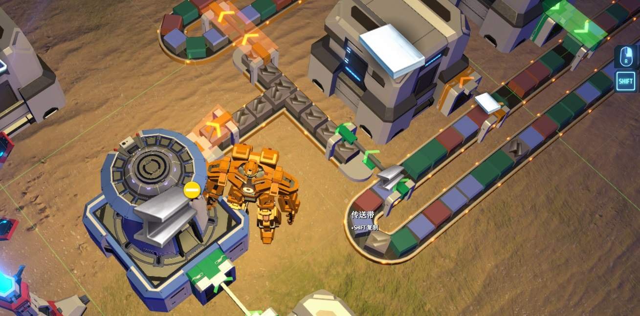
Basically, when the steel ratio in the belt loop is high and emptiness is low, the speed that we are getting steel from the belt loop is higher than the speed we deliver, as a result, the “horizontal” belt is always full. The product from the middle belt cannot get into the horizontal belt as long as it’s full.
Potential Caveat Discussion
Validity of the randomness model
This analysis is based on the assumption that the items on a belt will be randomly distributed. In reality it is more or less not so. Specifically, as player we tend build the same thing as the same place. As a result, the items on the belt is likely to exhibit some patterns thus deviate away from the math result based on random distribution.
At large scale belt loops though (main bus loop for mixed items), this tends to be a pretty good estimation. We might get somewhat higher ratio of one item and low ratio of another. But we can be sure that the big mixed item loop will never stop running and will contain each item type in a reasonable range.
Appendix: The elementary school Math
With independent random tests, to succeed the first one it takes, as expected value, 1/p runs.
In our case, the sorter returns and immediately does a “test” to try to deliver the item. So our Wait Time is effectively defined as number of tests – 1.
Note that, strictly speaking, the expected value of 1/X is not 1/E(X). That’s why I called it “estimated” efficiency instead of expected efficiency. They will be slightly off. But they should be close enough for estimation purposes.


Be the first to comment